The problem
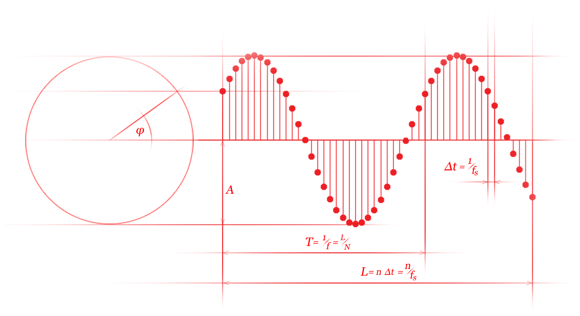
The equation of a sinusoid signal is a known fact:
$$y(t) = A \sin(2 \pi f t + \varphi) = A \sin(\omega t + \varphi).$$
However. This equation is only valid in the continuous time domain, therefore without any modification it is useless in the discrete time domain used by every digital machine. You won’t be able to create a continuous variable that spans through the duration of the signal from the beginning to the end while taking up every possible value.
Machines work with discrete time series that has a property called resolution. Resolution is the link between continous and discrete time domain. This property is implemented with sampling. It tells us how many data points were sampled equidistantly from the continuous signal within a time segment. In this way we can represent a continuous signal with discrete data points[1].
Therefore the t variable in the equation can be represented as a vector of data points. To create such a time vector, you have to choose a sampling interval.
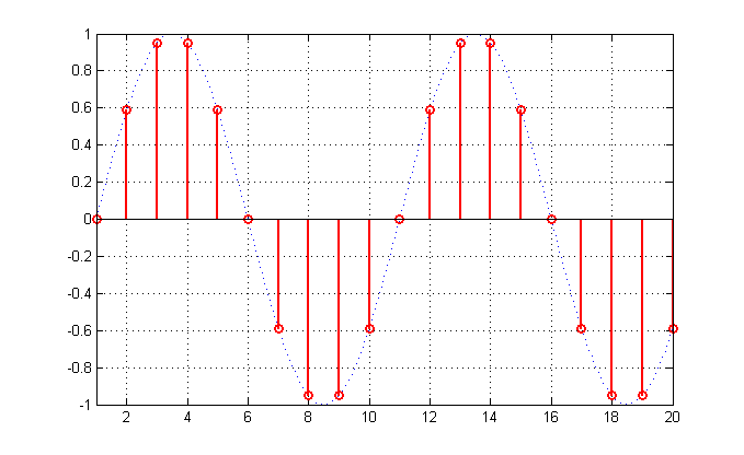
Let’s say you want to get 10 samples per seconds (fs=10Hz), and you want to have 20 samples in your vector. That also means that your time vector will cover almost 2 seconds[2] of continuous time.
You can test that the t1 and t2 vector are exactly the same. Both vector starts from zero and ends at 1.9. Having the time vector we can generate a sinusoid signal with a frequency of 1Hz. This will result 2 periods in the signal:
s = sin(2*pi*1*t1);
If we plot the generated signal, we can see, that it is not a sine signal at all. It is a discrete signal, that has values in discrete points as we expected.
This method is one of the 4 main signal generation methods where we link the discrete time signal to the continuous time. Having such a connection between the two domain, the signal can be played back with the computer’s digital to analog converter.
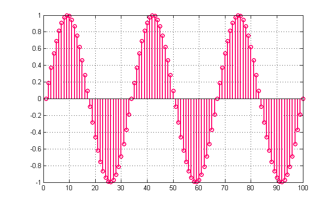
However. There are other use cases when we don’t want to link the discrete time to the continuous time, so we don’t have to bother with the sampling frequency, and we can generate a time vector from 0 to 1, and pass it to the equation:
t = linspace(0,1,100);
s = sin(2*pi*3*t);
The result will be a 100 sample long sinusoid signal, that contains 3 periods. But be careful. This signal can’t be used as the previous one until we specify the sampling frequency.
As you can see, generating sinusoids with these basic methods isn’t hard at all. But you have to think about the method, the formulas and the units. This could be a bit time consuming if you have to think about it every time you want to generate a signal…
Sinusoid signal parameters
There are 9 parameters that a pure sinusoid signal could have. In order to be able to generate any kind of sinusoid signals, you should be familiar with the parameters.
| Parameter name | Unit | Possible parameters |
|---|---|---|
phi |
[degree] | phase |
A |
[full scale] | amplitude[3] |
f |
[Hz] | frequency |
fs |
[Hz] | sample rate |
T |
[s] | period |
dt |
[s] | sample time |
L |
[s] | signal duration |
N |
[-] | number of periods |
n |
[-] | number of samples |
With these parameters there are 5 main generation methods for sinusoid signals. Each of them have alternatives that doesn’t count as an individual generation method due to the used parameters can be derived from the others if you apply the following formulas: fs = 1/dt, T = 1/f and L=n*dt.
| Method index | Required parameters | CT DT lock | Description |
|---|---|---|---|
| 1 | n N |
No | a signal consisting of n data points with Nperiods in it |
| 2 | L N fs |
Yes | L seconds long signal sampled at fs consisting of N periods in it |
| 3 | f N fs |
Yes | a signal sampled at fs sampling rate with N periods in it with the frequency f |
| 4 | f n fs |
Yes | a signal consisting of n data points sampled at fs sampling rate with the frequency f |
| 5 | f L fs |
Yes | a signal sampled at fs sampling rate with the duration of L seconds with the frequency f |
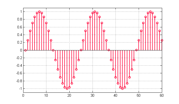
Let’s try out all methods, to see how you can use them in practice. Let’s generate the same 60 samples of sinusoid signal with 2.5 periods in it with the amplitude 1 at an arbitrary sampling frequency:
The used parameters may seem a bit odd for the first time, but due to the constraint of generating the same signal with all the methods, they will be reasonable.
Method 1 - [n,N]
Generating a sinusoid signal with n data points with N periods in it.
n = 60;
N = 2.5;
k = 0:n-1;
k = k/n;
s = sin(2*pi*N*k);
stem(s)
Method 2 - [L,N,fs]
Generating L seconds long signal sampled at fs consisting of N periods in it.
fs = 10;
N = 2.5;
L = 60/fs;
k = 0:1/fs:L-1/fs;
k=k/L;
s = sin(2*pi*N*k);
stem(s)
Method 3 - [f,N,fs]
Generating a sinusoid signal sampled at fs sampling rate with N periods in it with the frequency f.
fs = 10;
N = 2.5;
f = N*fs/60;
k = 0:1/fs:(N/f)-1/fs;
s = sin(2*pi*f*k);
stem(s)
Method 4 - [n,f,fs]
Generating a signal consisting of n data points sampled at fs sampling rate with the frequency f.
fs = 10;
n = 60;
f = 2.5*fs/n;
k = 0:n-1;
k = k*(1/fs);
s = sin(2*pi*f*k);
stem(s)
Method 5 - [f,L,fs]
Generating a sinusoid signal sampled at fs sampling rate with the duration of L seconds with the frequency f.
L = 60/fs;
f = 2.5/L;
n = 0:1/fs:L-1/fs;
s = sin(2*pi*f*n);
stem(s)
Summary
That’s it. These 5 methods cover all the possible non redundant ways to generate sinusoidal signals. Did you understand them? Did you like them? Will you use them? Will you study them? Will you derive them over and over again?
If your answers for the last two questions were both nope, then the go ahead and meet Smart Sinusoids.
Of course this is a very high level overview of the sampling theorem. There are much more detail how these things really work. ↩︎
Because we have started our time vector from 0 as the first vector point, the remained 19 points wont cover all the 2 seconds time duration but will span until 1.9 seconds (2s - 1/fs = 1.9s). ↩︎
PC sound cards usually accept signals scaled -1 to 1. ↩︎